Lecture 9

Indexes and external sorting

Overview

This lecture consists of three parts. In the first one we discuss basics of index structures along with their classification.

In the second one we present basic data structures for indexes.

In the third one we study the central problem for an operation on a database that of external sorting.

In the examples we use tables Emp and Dept known from SQL and PL/SQL lectures.

9.1 Indexes

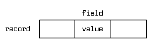
An index is a data structure on a disk, which allows for fast search of data in a database based on a search key value such as a person's name.

An index in a database has a similar meaning as an index in a book! In the simplest form the  search means: having a value we search for records which have this value in a given field.

Fig. 9.1 Searching for records by a value in a field
 

For example:

1. Show the data about a student with first name  'Harry'.
2. Show all students who are on the list of lecture 'Databases'.

Indexes are such data structures which help quickly find answers to such types of queries.

A search key for an index is a chosen record field or fields on the basis of which the search is to take place. An index is a data structure built out of nodes which contain the following forms of index records:

1. data entries k*  specified by the value of a search key k. There are three types of data entries (in every index there is only one type used):
   1. a data record with key value k,
   2. a pair: (k,w) where w is a pointer to the record with key value k,
   3. a pair: (k,w₁,...,w_n) where w is a list of pointers to records with key value k; an index record in this form is more compact than (ii) but requires a variable number of fields;
2. index entries which manage the process of finding the proper k* data entry based on the value k of the search key; an index entry can be for example a pair = (key value, pointer to a node in an index).

An index content is stored in a file called an index file.

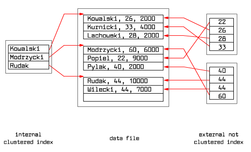
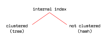
An index is called internal if its index file includes the data file, that is data entries are identical with data records, so we have to do with the case (1) above. An index which is not internal is called external.

An index is called clustered if both the data file and the data entries are sorted by the search key value of the index involved. As a result, records with the same or a close key value are located on the same page or only on a few disk pages. There may be only one clustered index because the data file may be sorted only by one search key values. An index, which is not clustered, is called unclustered.

Fig. 9.2 Two types of indexes

An index may be internal and unclustered. This is the case of the hash file.

When the search key includes the primary key then the index is called a primary index. When the search key includes a unique key then the index is called a unique index.

Composite search keys

Composite search keys are a combination of fields e.g. <sal,age>. The data entries order in an index with a composite key is based on lexicographical order.

Fig. 9.3 Single and composite search keys

On Figure 9.3, both the indexes with a complex search key support executing a query with the following WHERE clause: age=20 AND sal=75

And only the index with the key <age,sal> supports executing range queries with the following WHERE clauses: age<20 and age=20 AND sal>10

Let us look upon different types of indexes allowing for fast record search in a large record file.

9.2 Static ISAM tree (Indexed Sequential Access Method)

A popular method for a key search in a sorted file (in a sequence) is the binary search. We compare the searched key with the record's key located in the middle of a sequence and depending on the result of the comparison we search for the key either on the left hand side or on the right hand side of the sequence - using the described method recursively.

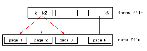
In the case of record storage on a disk, the binary search is easier if we use it not directly on the record file - but on the file which consists only of record keys k₁< k₂< … <k_N: where k_i is the lowest key on page i. The file with keys is an index file in this case.

Fig. 9.4 One level index file

The binary search is conducted on the much smaller index file and not on the record file! After finding the closest matching key we move to a page where a record of a given key is located - if it exists at all.

There is nothing against adding a new level of a sequential index with record keys to an index file - like in a sorted record sequence case. We can do this until we receive a single node and all levels of sequential indexes will together give us an index tree structure. We choose the number of elements in a node in such a way so that its content is written on one disk page. The resulting data structure is called an ISAM tree (ISAM is an abbreviation for Indexed Sequential Access Method).

Index page (tree node)

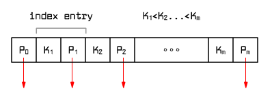
Fig. 9.5 Index page

An index page is a set of index entries <K_i,P_i> where K_i is a key and P_i is a pointer to a node at the next lower index level. The first element on the page is P₀ which is a pointer to a node at the next lower level. The following conditions are satisfied:

 

In the subtree pointed by P0 all the keys are < K1. In the subtree pointed by Pi all the keys are >=  Ki for i>=1. In the subtree pointed by Pi all the keys are < Ki+1 for i<m.

Figure 9.6 shows the rules for choosing branches when searching for a given key.

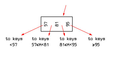
Fig. 9.6 Rules for choosing branches when performing a search
 

Figure 9.7 shows the structure of an ISAM tree.

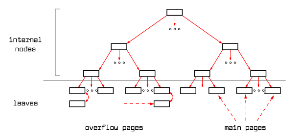
FIg. 9.7 ISAM tree structure
 

Example of an ISAM tree

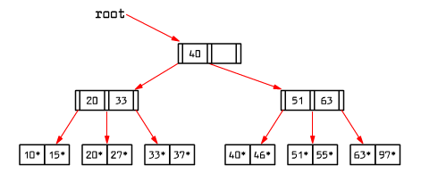
Fig. 9.8 Example of an ISAM tree
 

We insert 23*, 48*, 41*, 42*. We will receive an ISAM tree:

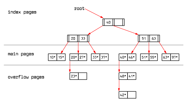
Fig. 9.9 ISAM tree after inserts
 

At the moment, since there is no free space on the primary pages, overflow pages are created and attached to the primary pages - creating unordered lists.

The structure of index pages and primary pages is fixed. If there is no more space on a primary page, overflow pages are attached to it. A situation may occur when one primary page will have a long list of overflow pages attached. Possibly, this makes a record search on such a list require to retrieve many pages into RAM and the process may take a while.

Summing up, ISAM trees are good for a record search based on its search key value or on the range of the search key values: A<= key <=B or A<= key or key <=B. If the number of records in a file is more or less fixed, ISAM structure is good. Since there is a risk that the keys will be clustered in sequences on overflow pages, this structure is not a stable one in a general case. Luckily its modification to the so called B+ trees exists which does not have its drawbacks.
 

9.3 B+ tree

B+ tree is a tree of an ISAM tree structure whose size changes dynamically depending on the number of data entries and where overflow pages are not used. B+ tree is height-balanced, that is, each leaf lies on the same depth in the tree. Moreover, the required occupancy of each of the index pages must be minimum 50% (excluding the root). Therefore each internal tree node (excluding the root) has m entries of an index (what corresponds to m+1 links down the tree such that:

d-1 <= m <= 2d-1

where d>=2 is a parameter called an order of B+ tree. The root has:

1 <= m <= 2d-1

index entries. Since the data entry's size may vary we do not set any condition on the number of data entries in a leaf besides that the occupancy of every leaf must be minimum 50%.

The maximum length of a path in a B+ tree from the root to a leaf is at most log_d N where N = #leaves. This brings us to a conclusion that the data entry search/insert/delete operations take on the order of log_d N of time.

The search begins at the root and the search key comparisons lead to a leaf, like in an ISAM tree.

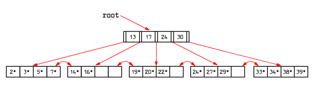
Fig. 9.10 B+ tree
 

To reach an entry with key = 5, we compare 5 with 13 at the root and choose the leftmost branch.

When searching for 15, at the root we find a proper branch to go down, that is the one between the keys 13 and 17. In the leaf we find only the elements 14 and 16. It means that element 15 is not available in this tree.

To check whether a given element is in a tree, we just have to follow the path starting from the root and ending in one of its leaves. All of the index pages on this path have to be retrieved to the RAM buffers.

To determine all the elements greater or equal to 24, first we find 24 (the smallest key greater than 24 or equal), then go right through all the leaves finding all the elements greater or equal to 24.

We assume that the tree leaves are located on the two-directional list structure - such a list helps to carry out range queries like the one above.

B+ tree as an internal and external index

As we described it above, an index may be internal and then the data entries coincide with the data records - this means that the data records are written into the B+ tree structure according to the search key order. Due to this fact, it is then a clustered index.

Or the index is external and then the data records are stored outside the index usually in no particular order.

Replacing frame strategy for B+ tree pages

An index is written into a file and its pages are retrieved to RAM buffers just like record pages with data. For an index file:

LRU is not a good method!

For B+ trees a better strategy is the following:

• it is better to keep the tree's root and the upper tree levels in RAM.

Additional operations on B+ trees

All commercial database management systems implement B+ trees although they usually do not remove physically index and data entries when they are deleted from the tree. On user's request or when the capacity in the tree falls down below a certain level - operation REBUILD is executed which recreates the index from the beginning or operation COALESCE which combines together neighboring pages of capacity below 50%.

If at the beginning we have a large set of records then, instead of repeating INSERT operations, it is better to use algorithm Bulk Loading which sorts records and then adds index levels above the sorted sequence, consecutively.

Why don't we use ordinary B trees?

To complete this topic, Fig. 9.11 shows a schema of a regular B tree (without +).

Fig. 9.11 An ordinary B tree node
 

Searching on ordinary B tree is faster. But because of the inconsistency of B tree nodes, operations INSERT and DELETE are more complicated. That is why in databases B+ trees are preferred.

 

Summary of trees Application of indexes of tree structure: range search, equality search, sort (e.g. ORDER BY), search with matching rows during joining of tables. ISAM tree – static structure: a simpler structure in comparison to B+ tree, only leaves are modified, overflow leaves are required – in pessimistic case they may have a bad impact on the time of executing SELECT statement unless we accept running operation REBUILD, sufficiently often. B+ tree – dynamic structure: in practice, height <=3, assuming that B+ tree root is always stored in RAM, the cost of a data entry search is of maximum 3 of I/O operations. This number will be used further on in our estimates.

9.4 Hash index

Hash index allows for fast search of records based on the search key value. It does not allow for range search.

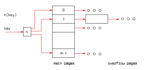
Hash index is a data structure based on placing data entries into buckets according to a hash function value of the search key. Each bucket consists of its primary page and possibly a list of overflow pages. The hash function value determines the bucket's primary page address where the record is to be searched for. In the case of larger number of records, overflow pages are created attached to the primary page.

Fig. 9.12 Hash index

 

If the hash function is properly chosen, almost all data entries are located on the primary page and there are no overflow pages (the average length of the overflow list is about 1.2). Therefore the average number of I/O operations for hash index when searching for a record is about 1.2. (We assume here that the bucket's address for a given hash function value is stored or can be calculated based on information stored in RAM.)

Hash function example:

h(k) = k mod M =  the bucket number to which every data entry with key k belongs (M = #buckets).

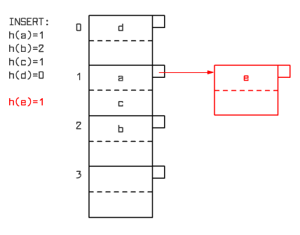
An example of hash index after performing a sequence of INSERT operations (with the assumption of 2 records on a page) is shown on Figure 9.13.

Fig. 9.13 Example of a hash index
 

We speak about static hashing when the number of buckets is set at the beginning and does not change. Along with the growth of the number of data entries (data records) the size of buckets increases and what follows, the search time increases which is proportional to the number of pages in a bucket. In the case of dynamic hashing the number of buckets adjusts dynamically to the number of data entries. Below there are mentioned two methods for dynamic hashing:

1. Periodic (e.g. once a day) rebuilding (REBUILD) of a hash file by changing the number of buckets. It is desired that a hash function has a feature of easy doubling the size of an index by splitting all of the buckets upon two. The function mod mentioned above has this property.

2. Extended hashing method

We avoid overflow pages by dynamic extension of bucket structures. An indirect catalogue directing to pages is used. When a bucket page is full, it is split upon two.

Internal hash index

Like in B+ trees it makes sense to speak about an internal hash index (data records are stored in an index) and about an external index (in the other case). When the search key = value condition results in a large number of data entries (in such a case we say that the condition is not selective; otherwise it is called selective), using an internal hash index will make the search significantly faster. In the case of hash index it makes no sense to speak about a clustered index because of random placing of records in the buckets.

Summarizing internal indexes

For one table there may be built practically only one internal index and many external indexes.

In an internal index built on a B+ tree the data records are stored on pages representing tree leaves. In an internal hash index the data records are stored on bucket pages. In both the cases, from the definitions of inserting and deleting algorithms, records can move between pages. It means that records may change pages so there can't be any pointers to them from the outside using page's identifier. As record's identifier, the value of its primary key is then used and the access to the record is performed through the primary index.

The primary index is either the same as the internal index under consideration or it is an external index where record identifiers are stored in its data entries. In the second case, when a record changes place (in the internal index) its identifier stored in the primary index also has to be updated.

Therefore building and using a clustered internal index makes search faster through this index - especially in the case of not selective search condition, e.g. range search; however the search of other indexes may become slower.

Fig. 9.14 Types of internal indexes

Multi-dimensional data structures

Up till now we have considered data structures which are one-dimensional - even if they are based on sets of values (vectors). Below there are two popular, easy index structures for multi-dimensional data.

(1) Grid file – partitioning of the search area, let us say located on the plane with horizontal and vertical lines, into rectangles. The points falling into one rectangle are stored in one bucket. When a bucket gets full we can then use overflow pages or split rectangles into smaller ones increasing the number of buckets.

(2) Partitioned hash function:

               H(v1,...,vn)=h1(v1)&h2(v2)&....&hn(vn)

The hash function value for a composite tuple is a concatenation of the hash function values for all its components.

9.5 External sort - multi-phase sort by merging

Let us consider the problem: sort 2GB of data in the RAM buffer of 100MB size. Classical methods of internal sort in RAM can not be directly used here.

In databases this type of sort problem happens often. Below there are examples:

1. ORDER BY clause - data are required in a particular order.
2. Construction of an initial B+ tree index (within methods BULK LOADING or REBUILD).
3. Joining of tables by using merge sort method.
4. Implementation of DISTINCT, GROUP BY, UNION and EXCEPT operators.

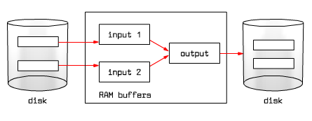
In the databases the method that is used, is called a multi-phase external sort by merging. The algorithm consists of two phases:

Phase 2: Multi-phase read of disk areas containing data, merge of consecutive blocks along with writing them into disk areas - repeated until we receive one single, ordered record block.

Fig. 9.15 Data block merge in the buffer pool
 

In each phase we read and write every page in the file.

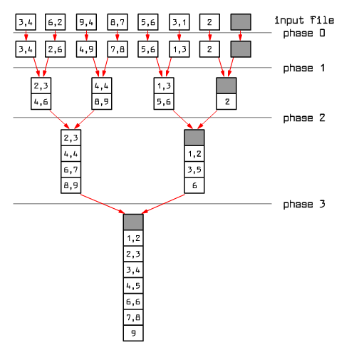
Fig.9.16 Example of the multi-phase external sort by merging

The number of I/O operations when executing external sort is <= 2N*#phases where N is the number of pages in a record file and factor 2 comes from the fact that we have to perform both read and write operations on every page.

In practice, the number of merge phases do not exceed 3. Together with the phase of building first blocks, the number of all phases is on average at most 4. Therefore the number of I/O operations needed to conduct the external sort is at most 8N (N is the number of pages in a record file).

External sort - using B+ trees

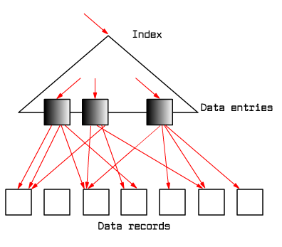
Let us assume that an index on B+ tree has been created on a record file. Is going through the leaves of this tree from the left hand side to the right hand side and writing all consecutive records a good sort method? Yes, but only when the index is clustered!

If the index is not clustered we must fetch to RAM the number of disk pages equal to the number of records (and not to how many pages records are stored in the file!) - which may result in a longer processing time than the time needed by the multi-phase sort by merging ~ 8N I/O operations where N is the number of pages in a record file.

Fig. 9.18 Illustration of a nonclustered index.

An advantage of the sort done by a B+ tree is its interactive character of receiving results. In comparison with internal sort, listing of results on user's screen may begin almost immediately without the necessity of waiting until the end. When the user is looking at the first portion of  results, the system may continue processing its next part.
 

9.7 Summary

During this lecture we have got acquainted with the details of index creation and of external sort.

9.8 Glossary

search key (record) - chosen record fields on the basis of which the search is to take place. There may be many search keys for a record.

index - data structure on a disk which allows for fast data search in a database based on record's search key, e.g. person's name. An index is saved into a file called an index file.

index file - file where index is stored.

internal index - an index whose file includes the data file that is the data entries in the index coincide with data records. It is also said that a table is organized by an index. In the other case, the index is called external.

external index - an index whose file is built independently of the data file, that is, the data entries are independent of data records.

clustered index - an index which organizes data entries and data records in an order by search key values. It means that records with the same or close key value are located on the same page or only a few disk pages. Otherwise we call an index unclustered. There may be only one clustered index and many unclustered ones.

primary index - a chosen index whose search key includes the primary key. There may be only one primary index.

unique index - an index whose search key includes a unique key. There may be many unique indexes.

ISAM tree - an index in the form of a static tree based on the binary search method.

B+ tree - an index in the form of a dynamic tree based on the binary search method.

hash index - an index in the form of a hash table.

external sort - a sort method for data which does not fit in RAM.

multi-phase external sort by merging - a basic method of external sort. There are two phases: creation of first ordered record blocks (called runs) - by using one of the internal sort methods and multi-phase read of these ordered record blocks which become larger and larger and their merge until one ordered block is obtained.

9.9 Exercises

1. Work out a dynamic hash algorithm expanding 1 and 2 idea shown during the lecture.