7.6 Rules of inference
Definition 7.6.1
Rules
of inference are schemes of the form
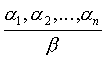
which assign the formula β to some
finite set of formulas α
1,..., α
n. We say that the rule of inference is correct iff
for
any structure STR such that STR |= α
1 ∧... ∧
α
n, holds STR |= β.
Formulas α
1,..., α
n are called rule's premisses and the formula β is called conclusion.
By definition, the correct rule of inference allows to deduce a
valid formula from the valid premisses. As in the case of propositional
calculus, one of the main predicate
calculus rules of inference is the rule of modus ponens. Other examples
of rules often applied in the mathematical proofs are: the rule
of generalization and the rule of introducing the existential
quantifier which we demonstrate below.
Lemma 7.6.1
For any formula α(x) and any formula β, the schema
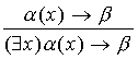
is a correct rule of inference, under assumption that no free
occurrence of x appears in β.
Proof.
Let's assume on the contrary that
(1) STR|= ( α(x) →
β
) and
(2) STR| ≠ (( ∃x)
α(x) → β).
Then from (2) for some valuation v we have STR,v|=( ∃x) α(x) i STR,v|= ¬ β. Hence, according
to the definition of semantics of quantifiers, for some a ∈ STR the following holds
STR, v(x/a)|= α(x)
STR, v(x/a)|= ¬ β
(because value of the variable x have no influence on the value of
formula β).
In consequence STR,v(x/a)|= ¬
(α(x) → β), contrary to (1).
We proved that the validity of the formula ( α(x)
→ β) implies the validity of the formula (( ∃ x) α(x) → β).
Lemma 7.6.2
For any formula α(x),

is the correct rule of inference (the rule of generalization).
Proof.
As soon as STR|= α(x),
then, regardless of the value of variable x (i.e. for every valuation
v),
we
obtain STR,v(a/x)|= α(x).
Hence STR, v|= ( ∀x)
α(x) for every v, finally STR|= ( ∀x)
α(x).
Notice, that if premisses of the correct rule of inference are
tautologies, then its conclusion is also a tautology. Thus, using
the well-know laws of predicate calculus and the correct rules of
inference
we may construct new interesting laws of predicate calculus.
Question 7.6.1: Are the
following rules of inference correct?
(a) The premiss: ( ∀x) ( α(x) → β(x)). The conclusion: (( ∀x)
α(x) →( ∀x) β(x)),
(b) The premiss: ( ∀x) ( α(x)
→ β(x)). The
conclusion: (( ∃x)
α(x) →( ∃x) β(x)),
(c) The premiss: (( ∃x)
α(x) ∧( ∃x) β(x)). The conclusion: ( ∃x) ( α(x) ∧ β(x)).
In what follows, we would like to present some applications of laws
as
well as rules of predicate calculus in proving problems.
Example 7.6.1
Let (Ai)i ∈
I be a family of subsets of set X and let f be a function f : X
→ Y. We prove that
f( ⎧⎫i ∈
I Ai) ⊆
⎧⎫
i ∈
I f(Ai).
Proof:
1. y ∈ f(⎧⎫
i ∈
I Ai) in accordance to the definition of
function's image
2. ( ∃ x ∈
X)( x ∈ ⎧⎫
i ∈
I Ai ∧ f(x)=y) from the
definition of generalized intersection operator
3. ( ∃ x ∈
X) (( ∀ i ∈
I) x ∈
Ai ∧ f(x)=y) from the law of
including-excluding
4. ( ∃ x ∈
X) ( ∀ i ∈
I) (x ∈
Ai ∧ f(x)=y) partial
commutability of quantifiers
5.( ∀ i ∈I) ( ∃ x ∈
X)(x ∈
Ai ∧ f(x)=y) from the
definition of function's image
6. ( ∀i ∈
I) y ∈ f(Ai) from the definition
of generalized intersection operator
7. y ∈ ⎧⎫
i ∈I f(Ai)
Let STR be an arbitrary data structure in which we interpret the
considered
formulas. We write shortly α ⇒ β to denote that if
α is true then β is also true in STR.
Similarly, we write α ≡
β to denote that the formula α
is semantically equivalent to the formula β
in the structure STR, i.e. if α
is true, then β is also true in the
structure STR and vice versa.
Using this notation we may write down the previously presented proof
in
the following form: 1 ≡ 2 ≡
3 ≡ 4 ⇒ 5 ≡ 6 ≡ 7. Hence, we
have proved 1 ⇒ 7.
Example 7.6.2
Let's consider the following theorem: In every linearly ordered set
<X, ≤ >, if x is a maximal element,
then it is
the largest element (see lecture 5).
Let x0 be the maximal element in the set X, then:
¬
( ∃x) (x0≤
x ∧ x≠ x0)
≡
(according to the law of de Morgan for quantifiers) ( ∀x)
¬ (x0≤
x ∧ x≠ x0)
≡ (according to de Morgan's law for
conjunction) (∀x) (¬
x0≤ x ∨
¬ x≠ x0)
≡ (because, by assumption, ≤ is a linear order) ( ∀x)
x≤ x0.
Of course, computer science also exploits rules of inference. If we
write a program, then it is recommended to give an argumentation that
this
program realizes its goals.
Example 7.6.3
Let a program's goal be to calculate the value of xn
where n and x are respectively the natural and real numbers. Assume
that we
are given the following program body (odd(m) means that m is an odd
natural
number).
{ z:= x; y :=1; m := n;
while (m > 0) {
if odd(m) { y := y * z; }
m := m div 2;
z := z * z;
}
}
Is this solution correct in the light of the given problem
specification?
We prove that if the initial value of the variable n is a natural
number,
then after program execution the value of the variable y is equal to
the n-th power of
x.
Regardless of the values of variables z, y and m, after the initial
assignments the following conjunction is satisfied (x =z
∧ m=n ∧ y=1).
Thus, before the first iteration of the loop "while" the
formula zm * y = xn is true.
Let us assume that this formula is satisfied during the i-th
entering
the loop. Notice, that the following formulas are valid in the set of
real
numbers:
( ∀m ∈N)(Odd(m) ∨ ¬ Odd(m)),
( ∀m ∈N)(Odd(m) → m=2*(m div2) + 1),
( ∀m ∈N)(¬
Odd(m) → m = 2*(m div2) ).
Hence, at the i-th entering the loop the below-mentioned
formula is also true
Odd(m) ∧ (z * z)m div 2
* (y * z) = xn &# ∨ ¬
Odd(m) ∧ (z * z)m div 2
* y = xn
If the value of m is an odd number before executing instruction "if"
(i.e.
the formula Odd(m) is true), then the next instruction {y := y *
z;} changes the value of the variable y. In consequence, after
executing the "if"-instruction (regardless of the test Odd(m) result)
the
formula (z * z)mdiv
2 * y = xn is satisfied. Now, as a result
of changing values of variables by instructions { m := m div 2; z := z
* z;} we obtain the valuation which satisfies the formula zm
*
y = xn. Thus, at the (i+1)-th entering the "while" loop
the condition zm * y = xn is
satisfied
again. It follows that the formula zm *
y = xn is true at the beginning of every iteration of
the loop.
Because at every iteration the variable m is divided by 2,
therefore,
after
a finite number of iterations the value of m will be equal to 0
(the set of natural numbers is well-founded, see lecture 5). Thus we
leave the "while" loop after a finite number of steps and the
resulting
valuation satisfies the condition (m=0 ∧
zm * y = xn), that is y = xn.
Conclusion: for any x ∈R and n ∈ N after program execution we have y = xn.